Data Wrangling
How do we do it? 🤔
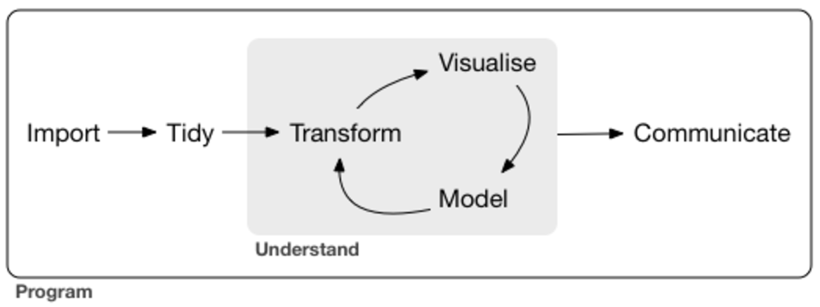
This diagram is taken from the R for Data Science book by Garrett Grolemund and Hadley Wickham, which it is a great resource for learning R. There is a whole community built around it and you could join it and start learning together: R4DS online learning community.
Dataset
To learn and practise how to organise data we will use a gapminder data set available from the gapminder package in R. This dataset is put into R by Jennifer Bryan from a tank of data sets available from Gapminder.
Gapminder is an independent Swedish foundation that helps to promote sustainable global development by collecting and analysing relevant data and by developing and designing teaching/learning tools. Gapminder was founded in Sweden by Hans Rosling who was a mastermind for distinctive and insightful storytelling about global development using visual animation.
You can see Hans in action in this BBC documentary The joy of Stats available on YouTube.
Gapminder Data
For each of 142 countries, the package provides values for life expectancy, GDP per capita, and population, every five years, from 1952 to 2007.
Before you can take a look at this data set first run the folowing code
# install necessary packages:
install.packages("dplyr", repos = "http://cran.us.r-project.org")
install.packages("ggplot2", repos = "http://cran.us.r-project.org")
install.packages("gapminder", repos = "http://cran.us.r-project.org")
# have a look at the data
head(gapminder::gapminder)## # A tibble: 6 x 6
## country continent year lifeExp pop gdpPercap
## <fct> <fct> <int> <dbl> <int> <dbl>
## 1 Afghanistan Asia 1952 28.8 8425333 779.
## 2 Afghanistan Asia 1957 30.3 9240934 821.
## 3 Afghanistan Asia 1962 32.0 10267083 853.
## 4 Afghanistan Asia 1967 34.0 11537966 836.
## 5 Afghanistan Asia 1972 36.1 13079460 740.
## 6 Afghanistan Asia 1977 38.4 14880372 786.💡Note that there are 6 columns, each of which we call a variable.
Description: Excerpt of the Gapminder data on life expectancy, GDP per capita, and population by country.
The main data frame gapminder has 1704 rows and 6 variables: - country: factor with 142 levels - continent: factor with 5 levels - year: ranges from 1952 to 2007 in increments of 5 years - lifeExp: life expectancy at birth, in years - pop: population - gdpPercap: GDP per capita
gapminder::gapminder[1:3,]## # A tibble: 3 x 6
## country continent year lifeExp pop gdpPercap
## <fct> <fct> <int> <dbl> <int> <dbl>
## 1 Afghanistan Asia 1952 28.8 8425333 779.
## 2 Afghanistan Asia 1957 30.3 9240934 821.
## 3 Afghanistan Asia 1962 32.0 10267083 853.1st look at the data using the following functions: dim() & head()
library(gapminder)
dim(gapminder)
## [1] 1704 6head(gapminder, n=10)## # A tibble: 10 x 6
## country continent year lifeExp pop gdpPercap
## <fct> <fct> <int> <dbl> <int> <dbl>
## 1 Afghanistan Asia 1952 28.8 8425333 779.
## 2 Afghanistan Asia 1957 30.3 9240934 821.
## 3 Afghanistan Asia 1962 32.0 10267083 853.
## 4 Afghanistan Asia 1967 34.0 11537966 836.
## 5 Afghanistan Asia 1972 36.1 13079460 740.
## 6 Afghanistan Asia 1977 38.4 14880372 786.
## 7 Afghanistan Asia 1982 39.9 12881816 978.
## 8 Afghanistan Asia 1987 40.8 13867957 852.
## 9 Afghanistan Asia 1992 41.7 16317921 649.
## 10 Afghanistan Asia 1997 41.8 22227415 635.Can you tell what each of the two functions does?!
Do we have the information about the structure of the data? 🤔 We can examine the structure using str() function, but the output could look messy and hard to follow if the data set is big. 🤪
str(gapminder) ## Classes 'tbl_df', 'tbl' and 'data.frame': 1704 obs. of 6 variables:
## $ country : Factor w/ 142 levels "Afghanistan",..: 1 1 1 1 1 1 1 1 1 1 ...
## $ continent: Factor w/ 5 levels "Africa","Americas",..: 3 3 3 3 3 3 3 3 3 3 ...
## $ year : int 1952 1957 1962 1967 1972 1977 1982 1987 1992 1997 ...
## $ lifeExp : num 28.8 30.3 32 34 36.1 ...
## $ pop : int 8425333 9240934 10267083 11537966 13079460 14880372 12881816 13867957 16317921 22227415 ...
## $ gdpPercap: num 779 821 853 836 740 ...The dplyr Package
The dplyr provides a “grammar” (the verbs) for data manipulation and for operating on data frames in a tidy way. The key operator and the essential verbs are:
%>%: the “pipe” operator used to connect multiple verb actions together into a pipeline.
select(): return a subset of the columns of a data frame.
mutate(): add new variables/columns or transform existing variables.
filter(): extract a subset of rows from a data frame based on logical conditions.
arrange(): reorder rows of a data frame according to single or multiple variables.
summarise() / summarize(): reduce each group to a single row by calculating aggregate measures.
We can have a look at the data and its structure by using the glimpse() function from the dplyr package.
suppressPackageStartupMessages(library(dplyr))
glimpse(gapminder)
## Observations: 1,704
## Variables: 6
## $ country <fct> Afghanistan, Afghanistan, Afghanistan, Afghanistan, Afghani…
## $ continent <fct> Asia, Asia, Asia, Asia, Asia, Asia, Asia, Asia, Asia, Asia,…
## $ year <int> 1952, 1957, 1962, 1967, 1972, 1977, 1982, 1987, 1992, 1997,…
## $ lifeExp <dbl> 28.801, 30.332, 31.997, 34.020, 36.088, 38.438, 39.854, 40.…
## $ pop <int> 8425333, 9240934, 10267083, 11537966, 13079460, 14880372, 1…
## $ gdpPercap <dbl> 779.4453, 820.8530, 853.1007, 836.1971, 739.9811, 786.1134,…🤓💡: Notice how we can prevent display of the messages that appear when uploading the packages by using, in this case, suppressPackageStartupMessages()!
Now we have the dplyr package uploaded, let us learn its verbs. 😇
The pipeline operater: %>%
Left Hand Side (LHS) %>% Right Hand Side (RHS)
x %>% f(…, y)
f(x,y)
The “pipe” **passes the result of the *LHS as the 1st operator argument of the function on the RHS**.
3 %>% sum(4) <==> sum(3, 4)
%>% is very practical for chaining together multiple dplyr functions in a sequence of operations.
Pick variables by their names: select(),
.png)
starts_with("X")every name that starts with “X”.ends_with("X")every name that ends with “X”.contains("X")every name that contains “X”.matches("X")every name that matches “X”, where “X” can be a regular expression.num_range("x", 1:5)the variables named x01, x02, x03, x04, x05.one_of(x)=> every name that appears in x, which should be a character vector.
👉 Practice ⏰💻: Select your variables
that ends with letter
pstarts with letter
co. Try to do this selection using base R.
😃🙌 Solutions:
gm_pop_gdp <- select(gapminder, ends_with("p"))
head(gm_pop_gdp, n = 1)
## # A tibble: 1 x 3
## lifeExp pop gdpPercap
## <dbl> <int> <dbl>
## 1 28.8 8425333 779.gm_cc <- select(gapminder, starts_with("co"))
head(gm_cc, n = 1)## # A tibble: 1 x 2
## country continent
## <fct> <fct>
## 1 Afghanistan Asiaof course all of this could be done using base R for example:
gm_cc <- gapminder[c("country", "continent")]but it’s less intuitive and often requires more typing.
Create new variables of existing variables: mutate()
.png)
It will allow you to add to the data frame df a new column, z, which is the multiplication of the columns x and y: mutate(df, z = x * y).
If we would like to observe lifeExp measured in months we could create a new column lifeExp_month:
gapminder2 <- mutate(gapminder, LifeExp_month = lifeExp * 12)
head(gapminder2, n = 2)
## # A tibble: 2 x 7
## country continent year lifeExp pop gdpPercap LifeExp_month
## <fct> <fct> <int> <dbl> <int> <dbl> <dbl>
## 1 Afghanistan Asia 1952 28.8 8425333 779. 346.
## 2 Afghanistan Asia 1957 30.3 9240934 821. 364.Pick observations by their values: filter()
.png)
There is a set of logical operators in R that you can use inside filter():
x < y:TRUEifxis less thanyx <= y:TRUEifxis less than or equal toyx == y:TRUEifxequalsyx != y:TRUEifxdoes not equalyx >= y:TRUEifxis greater than or equal toyx > y:TRUEifxis greater thanyx %in% c(a, b, c):TRUEifxis in the vectorc(a, b, c)is.na(x): IsNA!is.na(x): Is notNA
👉 Practice ⏰💻: Filter your data
Use gapminder2 df to filter:
only European countries and save it as
gapmEUonly European countries from 2000 onward and save it as
gapmEU21crows where the life expectancy is greater than 80
Don’t forget to use == instead of =! and
Don’t forget the quotes ""
😃🙌 Solutions:
gapmEU <- filter(gapminder2, continent == "Europe")
head(gapmEU, 2)
## # A tibble: 2 x 7
## country continent year lifeExp pop gdpPercap LifeExp_month
## <fct> <fct> <int> <dbl> <int> <dbl> <dbl>
## 1 Albania Europe 1952 55.2 1282697 1601. 663.
## 2 Albania Europe 1957 59.3 1476505 1942. 711.gapmEU21c <- filter(gapminder2, continent == "Europe" & year >= 2000)
head(gapmEU21c, 2)## # A tibble: 2 x 7
## country continent year lifeExp pop gdpPercap LifeExp_month
## <fct> <fct> <int> <dbl> <int> <dbl> <dbl>
## 1 Albania Europe 2002 75.7 3508512 4604. 908.
## 2 Albania Europe 2007 76.4 3600523 5937. 917.filter(gapminder2, lifeExp > 80)Reorder the rows: arrange()
is used to reorder rows of a data frame (df) according to one of the variables/columns.
.png)
If you pass
arrange()a character variable, R will rearrange the rows in alphabetical order according to values of the variable.If you pass a factor variable, R will rearrange the rows according to the order of the levels in your factor (running
levels()on the variable reveals this order).
👉 Practice ⏰💻: Arranging your data
1) Arrange countries in gapmEU21c df by life expectancy in ascending and descending order.
- Using
gapminder df
Find the records with the smallest population
Find the records with the largest life expectancy.
😃🙌 Solution 1):
gapmEU21c_h2l <- arrange(gapmEU21c, lifeExp)
head(gapmEU21c_h2l, 2)
## # A tibble: 2 x 7
## country continent year lifeExp pop gdpPercap LifeExp_month
## <fct> <fct> <int> <dbl> <int> <dbl> <dbl>
## 1 Turkey Europe 2002 70.8 67308928 6508. 850.
## 2 Romania Europe 2002 71.3 22404337 7885. 856.gapmEU21c_l2h <- arrange(gapmEU21c, desc(lifeExp)) # note the use of desc()
head(gapmEU21c_l2h, 2)## # A tibble: 2 x 7
## country continent year lifeExp pop gdpPercap LifeExp_month
## <fct> <fct> <int> <dbl> <int> <dbl> <dbl>
## 1 Iceland Europe 2007 81.8 301931 36181. 981.
## 2 Switzerland Europe 2007 81.7 7554661 37506. 980.😃🙌 Solution 2):
arrange(gapminder, pop)## # A tibble: 1,704 x 6
## country continent year lifeExp pop gdpPercap
## <fct> <fct> <int> <dbl> <int> <dbl>
## 1 Sao Tome and Principe Africa 1952 46.5 60011 880.
## 2 Sao Tome and Principe Africa 1957 48.9 61325 861.
## 3 Djibouti Africa 1952 34.8 63149 2670.
## 4 Sao Tome and Principe Africa 1962 51.9 65345 1072.
## 5 Sao Tome and Principe Africa 1967 54.4 70787 1385.
## 6 Djibouti Africa 1957 37.3 71851 2865.
## 7 Sao Tome and Principe Africa 1972 56.5 76595 1533.
## 8 Sao Tome and Principe Africa 1977 58.6 86796 1738.
## 9 Djibouti Africa 1962 39.7 89898 3021.
## 10 Sao Tome and Principe Africa 1982 60.4 98593 1890.
## # … with 1,694 more rowsarrange(gapminder, desc(lifeExp))## # A tibble: 1,704 x 6
## country continent year lifeExp pop gdpPercap
## <fct> <fct> <int> <dbl> <int> <dbl>
## 1 Japan Asia 2007 82.6 127467972 31656.
## 2 Hong Kong, China Asia 2007 82.2 6980412 39725.
## 3 Japan Asia 2002 82 127065841 28605.
## 4 Iceland Europe 2007 81.8 301931 36181.
## 5 Switzerland Europe 2007 81.7 7554661 37506.
## 6 Hong Kong, China Asia 2002 81.5 6762476 30209.
## 7 Australia Oceania 2007 81.2 20434176 34435.
## 8 Spain Europe 2007 80.9 40448191 28821.
## 9 Sweden Europe 2007 80.9 9031088 33860.
## 10 Israel Asia 2007 80.7 6426679 25523.
## # … with 1,694 more rowsCollapse many values down to a single summary: summarise()
.png)
The syntax of summarise() is simple and consistent with the other verbs included in the dplyr package.
uses the same syntax as
mutate(), but the resulting dataset consists of a single row instead of an entire new column in the case ofmutate().builds a new dataset that contains only the summarising statistics.
| Objective | Function | Description |
|---|---|---|
| basic | sum(x) |
Sum of vector x |
| centre | mean(x) |
Mean (average) of vector x |
median(x) |
Median of vector x | |
| spread | sd(x) |
Standard deviation of vector x |
quantile(x, probs) |
Quantile of vector x | |
range(x) |
Range of vector x | |
diff(range(x))) |
Width of the range of vector x | |
min(x) |
Min of vector x | |
max(x) |
Max of vector x | |
abs(x) |
Absolute value of a number x |
👉 Practice ⏰💻: Use summarise():
to print out a summary of gapminder containing two variables: max_lifeExp and max_gdpPercap.
to print out a summary of gapminder containing two variables: mean_lifeExp and mean_gdpPercap.
😃🙌 Solution: Summarise your data
summarise(gapminder, max_lifeExp = max(lifeExp), max_gdpPercap = max(gdpPercap))## # A tibble: 1 x 2
## max_lifeExp max_gdpPercap
## <dbl> <dbl>
## 1 82.6 113523.summarise(gapminder, mean_lifeExp = mean(lifeExp), mean_gdpPercap = mean(gdpPercap))## # A tibble: 1 x 2
## mean_lifeExp mean_gdpPercap
## <dbl> <dbl>
## 1 59.5 7215.Subsetting: group_by()
dplyr’s group_by() function enables you to group your data. It allows you to create a separate df that splits the original df by a variable.
The function summarise() can be combined with group_by().
| Objective | Function | Description |
|---|---|---|
| Position | first() | First observation of the group |
| last() | Last observation of the group | |
| nth() | n-th observation of the group | |
| Count | n() | Count the number of rows |
| n_distinct() | Count the number of distinct observations |
👉 Practice ⏰💻: Subset your data
- Identify how many countries are given in gapminder data for each continent.
😃🙌 Solution:
gapminder %>%
     group_by(continent) %>%
     summarise(n_distinct(country))
## # A tibble: 5 x 2
## continent `n_distinct(country)`
## <fct> <int>
## 1 Africa 52
## 2 Americas 25
## 3 Asia 33
## 4 Europe 30
## 5 Oceania 2Let’s %>% all up!
You can try to get into the habit of using a shortcut for the pipe operator

🗣👥 Confer with your neighbours:
What relationship do you expect to see between population size (pop) and life expectancy (lifeExp)?
Look what this code produces
gapminder_pipe <- gapminder %>%
  filter(continent == "Europe" & year ==  2007) %>%
  mutate(pop_e6 = pop / 1000000)
plot(gapminder_pipe$pop_e6, gapminder_pipe$lifeExp, cex = 0.5, col = "red")
tidyr
The tidyr can help you to create tidy data. Tidy data is data where:
- Every column is a variable
- Every row is an observation
- Every cell is a single value
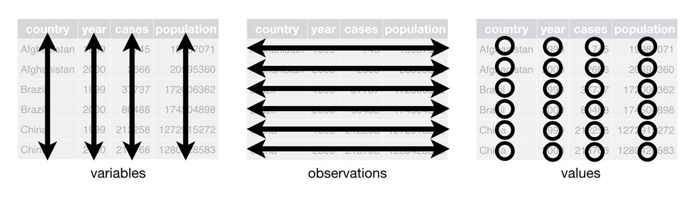
The tidyr package embraces the principles of tidy data and provides the standard key functionalities to organise data values within a dataset.
Hadley Wickham the author of the tidyr package talks in his paper Tidy Data about the importance of the data cleaning process and structuring datasets to facilitate data analysis.
Real datasets, that you are most likely to download from https://data.gov.rs/ or any other open source data platform, would often violate the three precepts of tidy data in all kinds of different ways:
- Variables would not have their names and column headers are values.
- A number of variables are stored in one column
- A single variable is stored in several columns
- Same information stored multiple times as different variables
to name a few.
To illustrate this, let us go back onto https://data.gov.rs/ and access Kvalitet Vazduha 2017. In particular, we want to access 2017-NO2.csv data.
## If you don't have tidyr installed yet, uncomment and run the line below
#install.packages("tidyr")
library(tidyr)
# access 2017-NO2.csv data
no2 <- read.csv("http://data.sepa.gov.rs/dataset/ca463c44-fbfa-4de9-9a75-790995bf2830/resource/74516688-5fb5-47b2-becc-6b6e31a24d80/download/2017-no2.csv",
                stringsAsFactors = FALSE,
                fileEncoding = "latin1")
# have a look at the data
glimpse(no2)
## Observations: 365
## Variables: 8
## $ Datum <chr> "01.01.2017", "02.01.2017", "03.01.2017", "04…
## $ Novi.Sad.SPENS.NO2 <dbl> 22.89, 32.94, 14.86, 22.73, 20.89, 10.47, 9.5…
## $ Beograd.Mostar.NO2 <dbl> 28.83, 39.12, 25.20, 28.48, 27.82, 41.91, 24.…
## $ Beograd.Vraèar.NO2 <dbl> 182.84, 244.56, 147.49, 159.12, 124.16, 42.17…
## $ Beograd.Zeleno.brdo.NO2 <dbl> 36.32, 36.68, 27.00, 35.15, 24.92, 8.27, 12.7…
## $ Kragujevac..NO2 <dbl> 38.92, 43.50, 40.17, 45.44, 43.04, 34.55, 25.…
## $ U.ice..NO2 <dbl> 49.84, 50.34, 36.35, 49.07, 33.33, 39.88, 33.…
## $ Ni..IZJZ.Ni...NO2 <dbl> 18.61, 22.87, 15.68, 21.97, 21.68, 12.11, NA,…It shows that this data set has 365 observations and 8 variables. Nonetheless, we need to consider what type of information we have here:
dateNO2 measurement taken: given in a single column -> ✅ tidy🙂placeswhere NO2 measurement was taken: given in several columns -> ❎ tidy🙁NO2measurements: given in several columns -> ❎ tidy🙁
Hmmm… 🤔 This doesn’t look tidy at all 😳
This data is about measurement level of NO2(µg/m3) in several different towns/places, which means that NO2 is our main response variable. The way in which this variable is given in this data is certainly not tidy. It defeats the key principles of tidy data: Every column is a variable and furthermore, Every row is NOT an observation.
It appears that this data has 8 variables, but we have realised that there are only 3: date, place and no2. To tidy it, we need to stack it by turning columns into rows. We are happy with the variable date and it should remain as a single column, the other 7 columns we want to convert into two variables: place and no2.
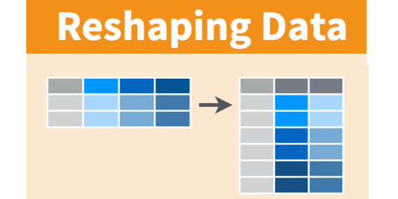
To make wide format data into tall format we have to turn columns into rows using gather() function.
We will create variable place in which we will hold the headers as given in the columns 2:8. The values inside those columns will be saved in the new variable no2.
new_no2 <- no2 %>%
  gather("place", "no2", -Datum, factor_key = TRUE) # stack all columns apart from `Datum`
glimpse(new_no2)
## Observations: 2,555
## Variables: 3
## $ Datum <chr> "01.01.2017", "02.01.2017", "03.01.2017", "04.01.2017", "05.01.…
## $ place <fct> Novi.Sad.SPENS.NO2, Novi.Sad.SPENS.NO2, Novi.Sad.SPENS.NO2, Nov…
## $ no2 <dbl> 22.89, 32.94, 14.86, 22.73, 20.89, 10.47, 9.58, 15.99, 14.46, 9…Let us see the names of the places
new_no2 %>%
     group_by(place) %>%
     summarise(n())
## # A tibble: 7 x 2
## place `n()`
## <fct> <int>
## 1 Novi.Sad.SPENS.NO2 365
## 2 Beograd.Mostar.NO2 365
## 3 Beograd.Vraèar.NO2 365
## 4 Beograd.Zeleno.brdo.NO2 365
## 5 Kragujevac..NO2 365
## 6 U.ice..NO2 365
## 7 Ni..IZJZ.Ni...NO2 365Those names look very messy. We could use function from stringr package str_sub(). To begin with let’s remove .NO2 at the end of each name.
## If you don't have stringr installed yet, uncomment and run the line below
#install.packages("stringr")
library(stringr)
new_no2$place <- new_no2$place %>%
    str_sub(end = -5)
glimpse(new_no2)
## Observations: 2,555
## Variables: 3
## $ Datum <chr> "01.01.2017", "02.01.2017", "03.01.2017", "04.01.2017", "05.01.…
## $ place <chr> "Novi.Sad.SPENS", "Novi.Sad.SPENS", "Novi.Sad.SPENS", "Novi.Sad…
## $ no2 <dbl> 22.89, 32.94, 14.86, 22.73, 20.89, 10.47, 9.58, 15.99, 14.46, 9…new_no2 %>%
group_by(place) %>%
summarise(n())## # A tibble: 7 x 2
## place `n()`
## <chr> <int>
## 1 Beograd.Mostar 365
## 2 Beograd.Vraèar 365
## 3 Beograd.Zeleno.brdo 365
## 4 Kragujevac. 365
## 5 Ni..IZJZ.Ni.. 365
## 6 Novi.Sad.SPENS 365
## 7 U.ice. 365It still doesn’t look right. 😟 This could be a tedious job. 😥 It is no wonder that many data analysts grumble about time spent on the process of cleaning and preparing the data. It could be a very long and time consuming process, but the more you do it and the more experience you gain the easier and less painful it gets.
Perhaps, you can try to explore other available packages in R that could help you with organising your data into your ideal format. To give you an idea we will show you how it can easily be done when using forcats::fct_recode() function.
## If you don't have forcats installed yet, uncomment and run the line below
#install.packages("forcats")
library(forcats)
new_no2 <- no2 %>%
  gather("place", "no2", -Datum, factor_key = TRUE) %>% # stack all columns apart from `Datum`
  mutate(place = fct_recode(place,
                            "NS_Spens" = "Novi.Sad.SPENS.NO2",
                            "BG_Most" = "Beograd.Mostar.NO2",
                            "BG_Vracar" = "Beograd.Vraèar.NO2",
                            "BG_ZelenoBrdo" = "Beograd.Zeleno.brdo.NO2",
                            "KG" = "Kragujevac..NO2",
                            "NI" = "Ni..IZJZ.Ni...NO2",
                            "UZ" = "U.ice..NO2"))
glimpse(new_no2)
## Observations: 2,555
## Variables: 3
## $ Datum <chr> "01.01.2017", "02.01.2017", "03.01.2017", "04.01.2017", "05.01.…
## $ place <fct> NS_Spens, NS_Spens, NS_Spens, NS_Spens, NS_Spens, NS_Spens, NS_…
## $ no2 <dbl> 22.89, 32.94, 14.86, 22.73, 20.89, 10.47, 9.58, 15.99, 14.46, 9…By now, you should have gained enough knowledge in using R to give you the necessary confidence to start exploring other functions of the tidyr package. You should not stop there, but go beyond and explore the whole of the tidyverse opinionated collection of R packages for data science. 😇🎶
To learn more about tidy data in r check Data Tidying section from the famous Data Science with R by Garrett Grolemund
Have you tried learning data science by posting your questions and discussing it with other people within the R community? 👥💻📊📈🗣 RStudio Community
YOUR TURN 👇
Practise by doing the following set of exercises:
Install and upload the
rattlepackage and see what it does.Create a new R script file to explore
weatherAUSdataset.
select()variable:MinTemp,MaxTemp,RainfallandSunshineby pipping the dataset into `dplyr::select() function.produce a summary using
base::summary()function of these numeric values.within this selection filter only those observations where
Rainfall >= 1and save the results into the computer’s memory (ie. save the results as an object).Try to think of how else you can use other
dplyrverbs on thisweatherAUSdataset. Write your question first, before embarking on typing the code.Write a short report on what visualisation you think would be interesting to produce for this
weatherAUSdataset and why?
Useful Links
Data Transformation with dplyr cheat sheet
© 2020 Sister Analyst