Basic Stats Concepts
In this section you will be introduced to a set of concepts that enable data to be explored with the objective
- of summarising and understanding the main features of the variables contained within the data and
- to investigate the nature of any linkages between the variables that may exist
The starting point is to understand what data is.
- What is the population?
- Why do we use samples?
Can you provide a formal definition of the population and the sample? 😁
The population is the set of all people/objects of interest in the study being undertaken.
In statistical terms the whole data set is called the population. This represents “Perfect Information”, however in practice it is often impossible to enumerate the whole population. The analyst therefore takes a sample drawn from the population and uses this information to make judgements (inferences) about the population.
Clearly if the results of any analysis are based on a sample drawn from the population, then if the sample is going to have any validity, then the sample should be chosen in a way that is fair and reflects the structure of the population.
The process of sampling to obtain a representative sample is a large area of statistical study. The simplest model of a representative sample is a “random sample”:
A sample chosen in such a way that each item in the population has an equal chance of being included in the sample.
As soon as sample data is used, the information contained within the sample is “Imperfect” and depends on the particular sample chosen. The key problem is to use this sample data to draw valid conclusions about the population with the knowledge of and taking into account the ‘error due to sampling’.
The importance of working with representative samples should be seriously considered; a good way to appreciate this importance is to see the consequences of using unrepresentative samples. A book by Darrell Huff called How to Lie with Statistics, published by Penguin contains several anecdotes of unrepresentative samples and the consequences of treating them as representative.
Data Analysis Using Sample Data
Usually the data will have been collected in response to some perceived problem, in the hope of being able to glean some pointers from this data that will be helpful in the analysis of the problem. Data is commonly presented to the data analyst in this way with a request to analyse the data.
Before attempting to analyse any data, the analyst should:
Make sure that the problem under investigation is clearly understood, and that the objectives of the investigation have been clearly specified.
Before any analysis is considered the analyst should make sure that the individual variables making up the data set are clearly understood.
The analyst must understand the data before attempting any analysis.
In the summary you should ask yourself:
Do I understand the problem under investigation and are the objectives of the investigation clear? The only way to obtain this information is to ask questions, and keep asking questions until satisfactory answers have been obtained.
Do I understand exactly what each variable is measuring/recording?
Describing Variables
A starting point is to examine the characteristics of each individual variable in the data set.
The way to proceed depends upon the type of variable being examined.
Classification of variable types
The variables can be one of two broad types:
- Attribute variables: are variables that have their outcomes described in terms of their characteristics or attributes.
- gender
- days in a week
A common way of handling attribute data is to give it a numerical code. Hence, we often refer to them as coded variables.
- Measured variables: are variables that have their outcomes taken from a numerical scale; the resulting outcome is expressed in numerical terms.
- weight
- age
There are two types of measured variables, a measured variable that is measured on some continuous scale of measurement, e.g. a person’s height. This type of measured variable is called a continuous variable. The other type of measured variable is a discrete variable. This results from counting; for example ‘the number of passengers on a given flight’.
The Concept of Statistical Distribution
The concept of statistical distribution is central to statistical analysis.
This concept relates to the population and conceptually assumes that we have perfect information, the exact composition of the population is known.
The ideas and concepts for examining population data provide a framework for the way of examining data obtained from a sample. The Data Analyst classifies the variables as either attribute or measured and examines the statistical distribution of the particular sample variable from the sample data.
For an attribute variable the number of occurrences of each attribute is obtained, and for a measured variable the sample descriptive statistics describing the centre, width and symmetry of the distribution are calculated.
attribute:
measured:
What does the distribution show?
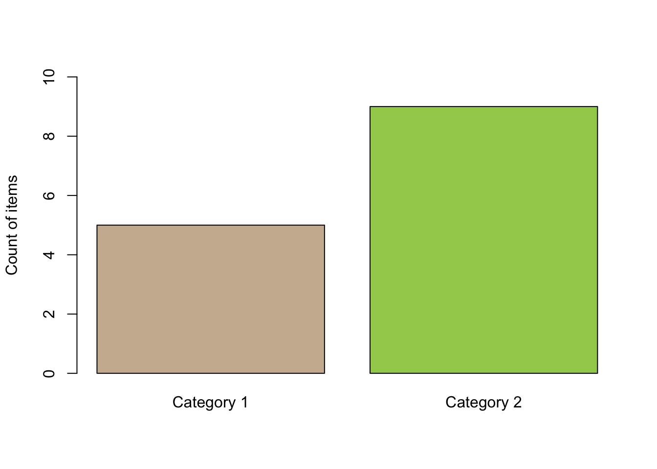
For an attribute variable it is very simple. We observe the frequency of occurrence of each level of the attribute variable as shown in the barplot above.
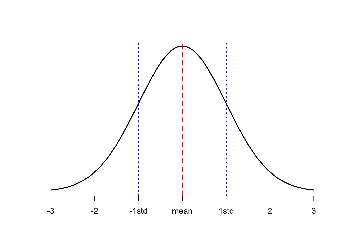
For a measured variable the area under the curve from one value to another measures the relative proportion of the population having the outcome value in that range.
A statistical distribution for a measured variable can be summarised using three key descriptions:
- the centre of the distribution;
- the width of the distribution;
- the symmetry of the distribution
The common measures of the centre of a distribution are the Mean (arithmetic average) and the Median. The median value of the variable is defined to be the particular value of the variable such that half the data values are less than the median value and half are greater.
The common measures of the width of a distribution are the Standard Deviation and the Inter-Quartile Range. The Standard Deviation is the square root of the average squared deviation from the mean. Ultimately the standard deviation is a relative measure of spread (width), the larger the standard deviation the wider the distribution. The inter-quartile range is the range over which the middle 50% of the data values varies.
By analogy with the median it is possible to define the quartiles:
- Q1 is the value of the variable that divides the distribution 25% to the left and 75% to the right.
- Q2 is the value of the variable that divides the distribution 50% to the left and 50% to the right. This is the median by definition.
- Q3 is the value of the variable that divides the distribution 75% to the left and 25% to the right.
- The inter-quartile range is the value Q3 - Q1.
The diagram below shows this pictorially:

🤓💡 Conventionally the mean and standard deviation are given together as one pair of measures of location and spread, and the median and inter-quartile range as another pair of measures.
There are a number of measures of symmetry; the simplest way to measure symmetry is to compare the mean and the median. For a perfectly symmetrical distribution the mean and the median will be exactly the same. This idea leads to the definition of Pearson’s coefficient of Skewness as:
Pearson's coefficient of Skewness = 3(mean - median) / standard deviation
An alternative measure of Skewness is the Quartile Measure of Skewness defined as:
Quartile Measure of Skewness = [(Q1 - Q3) - (Q2 - Q1)]/(Q3 - Q1)
Important Key Points:
- What is Data?
- Variables
- Two types of variable:
- an attribute variable
- a measured variable
- The concept of Statistical Distribution:
- As applied to an attribute variable
- As applied to a measured variable
- Descriptive Statistics for a measured variable:
- Measures of Centre
- Mean, Median
- Measures of Width:
- Standard Deviation
- Inter-Quartile Range
- Measures of Centre
The descriptive statistics provide a numerical description of the key parameters of the distribution of a measured sample variable.
Investigating the relationship between variables
One of the key steps required of the Data Analyst is to investigate the relationship between variables. This requires a further classification of the variables contained within the data, as either a response variable or an explanatory variable.
A response variable is a variable that measures either directly or indirectly the objectives of the analysis.
An explanatory variable is a variable that may influence the response variable.
Bivariate Relationships
In general there are four different combinations of type of Response Variable and type of Explanatory Variable. These four combinations are shown below:
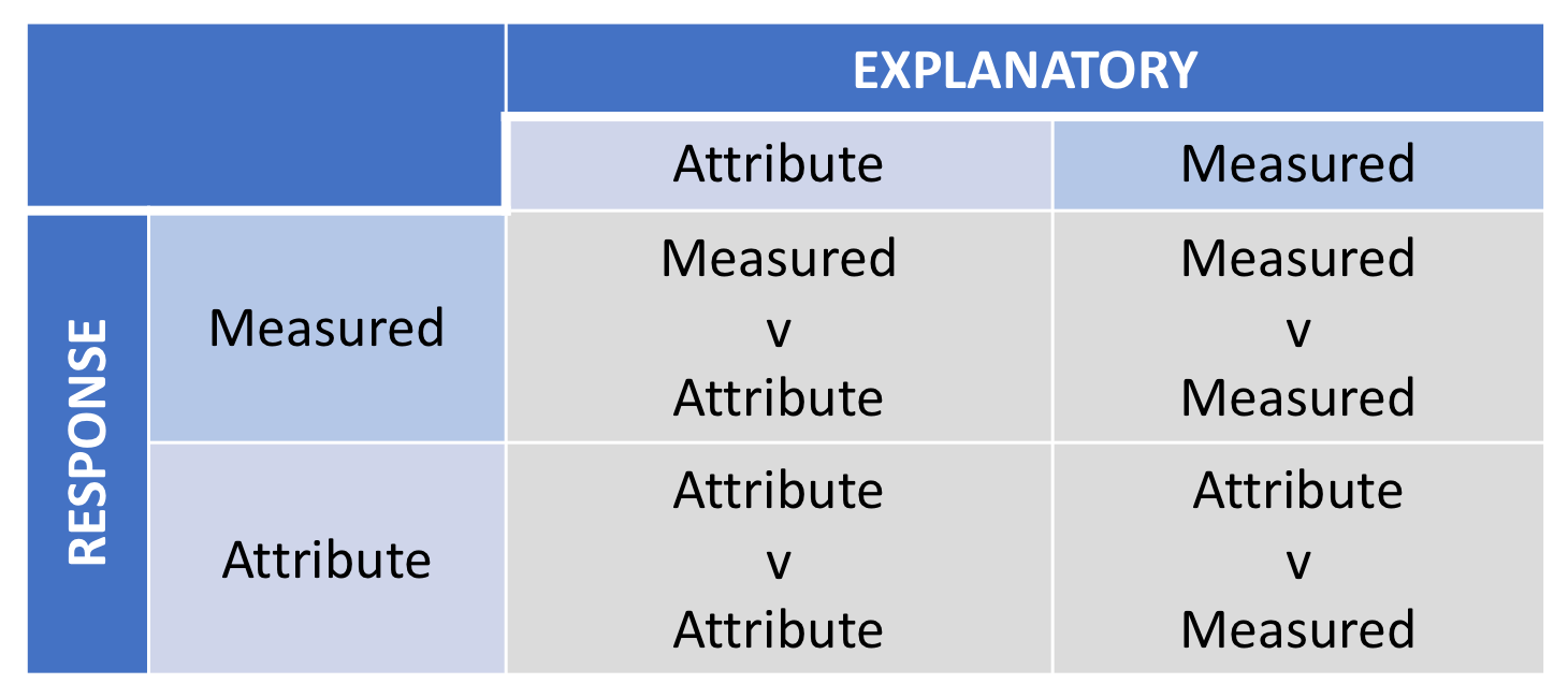
DA Matrix
The starting point for any investigation of the connections between a response variable and an explanatory variable starts with examining the variables, and defining the response variable, or response variables, and the explanatory variables.
🤓💡: In large empirical investigations there may be a number of objectives and a number of response variables.
The method for investigating the connections between a response variable and an explanatory variable depends on the type of variables. The methodology is different for combinations as shown in the box above, and applying an inappropriate method causes problems. 💡⚡️😩
DA Methodology
The first step is to have a clear idea of what is meant by a connection between the response variable and the explanatory variable. This will provide a framework for defining a Data-Analysis process to explore the connection between the two variables, and will utilise the ideas previously developed.
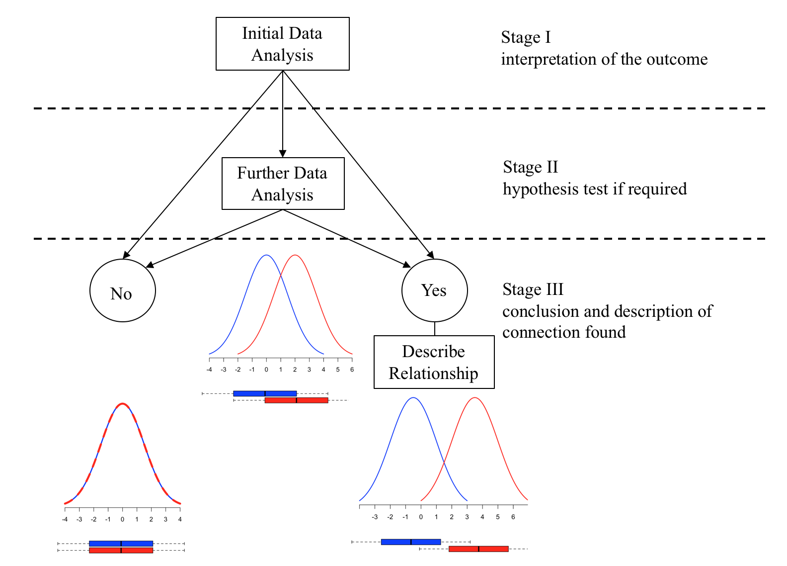
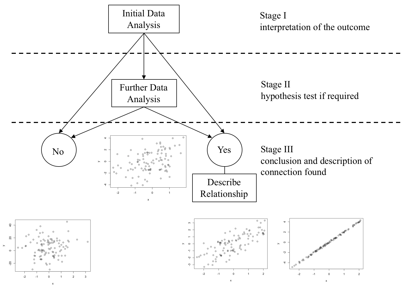
The next step is to use some simple sample descriptive statistics to have a first look at the nature of the link between the variables. This simple approach may allow the analyst to conclude that on the basis of the sample information there is strong evidence to support a link, or there is no evidence of a link, or that the simple approach is inconclusive and further more sophisticated data analysis is required. This step is called the Initial Data Analysis and sometimes abbreviated to IDA.
If the Initial Data Analysis suggests that Further Data Analysis (FDA) is required, then this step seeks one of two conclusions:
- The sample evidence is consistent with there being no link between the response variable and the explanatory variable.
or
- The sample evidence is consistent with there being a link between the response variable and the explanatory variable.
The outcome of the analysis is one of the two alternatives given above. If the outcome is that there is no evidence of a connection, then no further action is required by the analyst since the analysis is now complete.
If however the outcome of the analysis is that there is evidence of a connection, then the nature of the connection between the two variables needs to be described.
🤓💡 The Data-Analysis Methodology described above seeks to find the answer to the following key question:
On the basis of the sample data is there evidence of a connection between the response variable and the explanatory variable?
The outcome is one of two conclusions
No evidence of a relationship
Yes there is evidence of a relationship, in which case the link needs to be described.
This process can be represented diagrammatically as:

For each of the four data analysis situations given, the data analyst needs to know what constitutes the Initial Data Analysis (I.D.A.) and how to undertake and interpret the I.D.A. If Further Data Analysis is required the analyst needs to know how to undertake and interpret the Further Data Analysis.
Measured Vs Attribute(2-levels)
There is a relationship between a measured response and an attribute explanatory variable if the average value of the response is dependent on the level of the attribute explanatory variable.
Given a measured response and an attribute explanatory variable with two levels, “red” & “blue”, if the statistical distribution of the response variable for attribute level “red” and attribute level “blue” are exactly the same then the level of the attribute variable has no influence on the value response, there is no relationship.
This can be illustrated as below:
Red variant
Measured Vs Measured
The first step is to have a clear idea of what is meant by a connection between a measured response variable and a measured explanatory variable. Imagine a population under study consisting of a very large number of population members, and on each population member two measurements are made, the value of \(Y\) the response variable and the value of \(X\) the explanatory variable. For the whole population a graph of \(Y\) against \(X\) could be plotted conceptually.
If the graph shows a perfect line, then there is quite clearly a link between \(Y\) and \(X\). If the value of \(X\) is known, the exact value of \(Y\) can be read off the graph. This is an unlikely scenario in the data-analysis context, because this kind of relationship is a deterministic relationship. Deterministic means that if the value of \(X\) is known then the value of Y can be precisely determined from the relationship between Y and \(X\). What is more likely to happen is that other variables may also have an influence on \(Y\).
If the nature of the link between Y and X is under investigation then this could be represented as:
\(Y = f(X) + effect\) of all other variables [effect of all other variables is commonly abbreviated to \(e\)]
Considered the model:
\[Y = f(X) + e \text{ [e is the effect of all other variables]}\]
The influence on the response variable Y can be thought of as being made up of two components:
the component of Y that is explained by changes in the value of X, [the part due to changes in \(X\) through \(f(X)\)]
the component of Y that is explained by changes in the other factors. [the part not explained by changes in \(X\)]
Or in more abbreviated forms the ‘Variation in Y Explained by changes X’ or ‘Explained Variation’ and the ‘Variation in Y not explained by changes in X’ or the ‘Unexplained Variation’.
In conclusion, the Total Variation in Y is made up of the two components:
- the \(Changes in Y Explained by changes in X\) and
- the \(Changes in Y not explained by changes in X\)
Which may be written as:
\[\text{The Total Variation in Y = Explained Variation + Unexplained Variation}\]
🤓💡 The discussion started with the following idea:
\[Y = f(X) + e\]
And to quantify the strength of the link the influence on \(Y\) was broken down into two components:
$$\text{The Total Variation in Y = Explained Variation + Unexplained Variation}$$This presents two issues:
A: Can a model of the link be made? B. Can The \(Total Variation in Y\), \(Explained Variation\) and the \(Unexplained Variation\) be measured?
What do these quantities tell us?
Maybe we can observe a proportion of the \(Explained Variation in Y\) over the \(Total Variation in Y\). This ratio is always on the scale \(0\) to \(1\), but by convention is usually expressed as a percentage so is regarded as on the scale \(0\) to \(100\%\). It is called \(R^2\) and interpretation of this ratio is as follows:
\[R^2: 0\% \text{ (no link) <--------------- } 50\% \text{(Statistical Link) ---------------> }100\%\text{ (Perfect Link)}\]
The definition and interpretation of R_sq is a very important tool in the data analyst’s tool kit for tracking connections between a measured response variable and a measured explanatory variable.
We can put those ideas into our DA Methodology frameworks as shown below.
Red variant
🤓💡 Note that you will hardly ever be in the situation in which \(R^2\) would be so close to zero that would make you conclude that on the basis of the sample evidence used in IDA it is possible to conclude that there is no relationship between the two variables. If \(R^2\) value is very small (for example around \(2\%\)) this would need to be further tested to conclude if it is statistically significant based on the sample evidence by applying FDA.
Further Data Analysis
If the ‘Initial Data Analysis’ is inconclusive then ‘Further Data Analysis’ is required.
The ‘Further Data Analysis’ is a procedure that enables a decision to be made, based on the sample evidence, as to one of two outcomes:
- There is no relationship
- There is a relationship
These statistical procedures are called hypothesis tests, which essentially provide a decision rule for choosing between one of the two outcomes: “There is no relationship” or “There is a relationship” based on the sample evidence.
All hypothesis tests are carried out in four stages:
Stage 1: Specifying the hypotheses.
Stage 2: Defining the test parameters and the decision rule.
Stage 3: Examining the sample evidence.
Stage 4: The conclusions.
Statistical Models used in FDA
Measured Response v Attribute Explanatory Variable with exactly two levels:
- t-test
Measured Response v Attribute Explanatory Variable with more than two levels:
- One-Way ANOVA
Measured Response v Measured Explanatory Variable
- Simple Regression Model
- Measured Response v Measured Explanatory Variables
- Multifactor Regression Model
- Attribute Response v Attribute Explanatory Variable
- Chi-Square Test of Independence
YOUR TURN 👇
Make sure you can answer the following questions:
What are the underlying ideas that enable a relationship between two variables to be investigated?
What is the purpose of summary statistics?
What is the data analysis methodology for exploring the relationship between:
a measured response variable and an attribute explanatory variable?
a measured response variable and a measured explanatory variable?
© 2020 Sister Analyst